Motor coefficients
In this section, you will experimentally identify the electric motor model coefficients.
Theoretical background
PWM (Pulse-Width Modulation) is a technique used to control the average power delivered by a digitally switched signal. By rapidly switching the signal between its maximum value and zero (on-off) and varying the fraction of time the signal stays at its maximum (duty cycle), you can control the average power delivered to the load (i.e., by modulating the pulse width).


This is the mechanism used by the Crazyflie to drive its motors. In code you can set a real value between 0.0 and 1.0, which corresponds to the motor PWM.
You will implement a function that, given a desired angular velocity, computes the corresponding PWM value.
Experimental procedure
To measure the propeller angular velocity, you will use a tachometer. The tachometer detects the interruption of light when the propeller blade crosses its light beam. The rotational speed is then computed by counting how many times this happens within a given time interval.
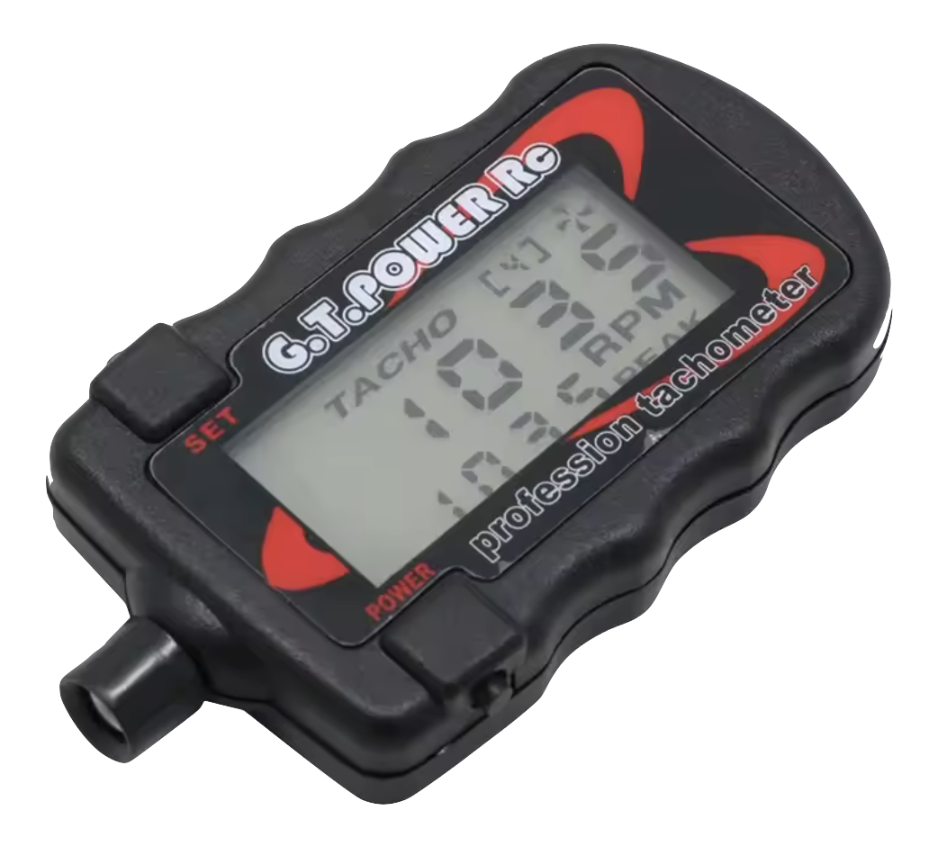
The POWER button turns on the devide, while the SET button configure the number of blades of the propeller. The screen will display the current angular velocity in \(\text{rpm}\), while the maximum value will be memorized as "peak" data at the bottom.
You must flash a program to the drone that turns on only one motor using a chosen PWM value. You will collect propeller angular velocity data for 10 distinct PWM values. For each PWM value, repeat the experiment 3 times and compute the average.

To simplify the procedure, you can change the PWM command using the Up and Down buttons in the Command Based Flight Control, located at the bottom-right corner of the Crazyflie Client.

Create a file named motor_coefficients.c inside src/identification with the following code:
#include "FreeRTOS.h"      // FreeRTOS core definitions (needed for task handling and timing)
#include "task.h"          // FreeRTOS task functions (e.g., vTaskDelay)
#include "supervisor.h"    // Functions to check flight status (e.g., supervisorIsArmed)
#include "commander.h"     // Access to commanded setpoints (e.g., commanderGetSetpoint)
#include "motors.h"        // Low-level motor control interface (e.g., motorsSetRatio)

// Global variables to store the desired setpoint, the current state (not used here) and the computed PWM value.
setpoint_t setpoint;
state_t state;
float pwm;

// Main application
void appMain(void *param)
{
    // Infinite loop (runs forever)
    while (true)
    {
        // Check if the drone is armed (i.e., ready to fly)
        if (supervisorIsArmed())
        {
            // Fetch the latest setpoint from the commander and also fetch the current estimated state (not used here)
            commanderGetSetpoint(&setpoint, &state);

            // Compute a PWM value proportional to the commanded altitude (Z axis position)
            // The altitude command increases in 0.5 m steps, and we want the PWM to increase by 0.1 for each step.
            // Therefore, we divide Z by 5.0 so that: 0.5 m → 0.1 PWM
            pwm = (setpoint.position.z) / 5.0f;
        }
        else
        {
            // If not armed, stop the motor (set PWM to zero)
            pwm = 0.0f;
        }
        // Send the PWM signal to motor M1, scaling it to match the expected range [0, UINT16_MAX]
        motorsSetRatio(MOTOR_M1, pwm * UINT16_MAX);
        // Wait for 100 milliseconds before running the next iteration (10 Hz control loop)
        vTaskDelay(pdMS_TO_TICKS(100));
    }
}
Follow these measurement steps:
- Ensure that the drone battery is fully charged
- Fix the drone at the table using masking tape
- Arm the drone by pressing the Arm button in the Crazyflie Client
- Turn on the motor at a specific PWM value using Up and Down buttons in the Command Based Flight Control
- Turn on the tachometer by clicking POWER
- Point the tachometer at the propeller from approximately \(30~\text{cm}\) away
- Write down the peak data shown on the display
- Repeat steps 1–7 for the other PWM values
After the experiment, fill in the table below:
| \({\color{var(--c3)}PWM}\) | \({\color{var(--c1)}\omega_1}~(\text{rad/s})\) | \({\color{var(--c1)}\omega_2}~(\text{rad/s})\) | \({\color{var(--c1)}\omega_3}~(\text{rad/s})\) |
|---|---|---|---|
0.1 |
|||
0.2 |
|||
0.3 |
|||
0.4 |
|||
0.5 |
|||
0.6 |
|||
0.7 |
|||
0.8 |
|||
0.9 |
|||
1.0 |
Data analysis
Using the collected data, we should fit a curve relating the propeller angular velocity \({\color{var(--c1)}\omega}\)(1) with the corresponding \({\color{var(--c3)}PWM}\) command.
- Note that you must convert from \(\text{rpm}\) to \(\text{rad/s}\)

There are many possible fitting models (linear, exponential, polynomial, etc.):
To decide which one is most appropriate here, we need to look more closely at the system dynamics. A simplified electromechanical model of an electric motor driving a propeller is shown below(1).
- Although the Crazyflie uses a brushless DC motor (BLDC), its mathematical model at steady state is equivalent to a brushed DC motor.

Where:
- \({\color{var(--c3)}e_a}\) — Armature voltage (\(\text{V}\))
- \({\color{var(--c2)}i_a}\) — Armature current (\(\text{A}\))
- \({\color{var(--c1)}e_b}\) — Back-EMF voltage (\(\text{V}\))
- \({\color{var(--c2)}\tau_m}\) — Motor torque (\(\text{N.m}\))
- \({\color{var(--c1)}\omega}\) — Motor/propeller angular velocity (\(\text{rad/s}\))
- \(R_a\) — Armature resistance (\(\Omega\))
- \(L_a\) — Armature inductance (\(\text{H}\))
- \(k_d\) — Propeller drag constant (\(\text{N.m.s}^2\text{/rad}^2\))
- \(b\) — Viscous friction coefficient (\(\text{N.m.s/rad}\))
- \(I\) — Motor/propeller moment of inertia (\(\text{kg.m}^2\))
Exercise 1
Apply Kirchhoff’s voltage law (KVL) to the armature circuit.
Answer
Exercise 2
Apply Newton’s second law for rotation about the motor shaft.
Answer
For a DC motor, the motor torque \({\color{var(--c2)}\tau_m}\) is directly proportional to the armature current \({\color{var(--c2)}i_a}\), and the back-EMF voltage \({\color{var(--c1)}e_b}\) is directly proportional to the angular velocity \({\color{var(--c1)}\omega}\):
Where:
- \(K_m\) - Motor torque constant (\(\text{N.m/A}\) or \(\text{V.s/rad}\)).
Exercise 3
Substitute \({\color{var(--c2)}\tau_m}\) and \({\color{var(--c1)}e_b}\) into the two differential equations obtained above.
Answer
When the motor reaches steady state, the armature current \({\color{var(--c2)}i_a}\) and angular velocity \({\color{var(--c1)}\omega}\) become constant (this is what “steady state” means):
Exercise 4
Set the derivatives of \({\color{var(--c2)}i_a}\) and \({\color{var(--c1)}\omega}\) to zero and isolate \({\color{var(--c2)}i_a}\) in both equations.
Answer
Exercise 5
Equate the two expressions for \({\color{var(--c2)}i_a}\) and isolate the armature voltage \({\color{var(--c3)}e_a}\).
Answer
The \({\color{var(--c3)}\text{PWM}}\) command is the ratio between the armature voltage \({\color{var(--c3)}e_a}\) and the battery supply voltage \(e_s\):
Exercise 6
Substitute \({\color{var(--c3)}e_a}\) into the equation above and isolate \({\color{var(--c3)}PWM}\).
Answer
You should obtain:
Since \(R_a\), \(k_d\), \(b\), \(K_m\), and \(e_s\) are constant, we can group them into two coefficients:
That is, the most appropriate curve fit here is a second-order polynomial with zero constant term:
So, instead of identifying each physical parameter (\(R_a\), \(k_d\), \(b\), \(K_m\), and \(e_s\)), you will experimentally identify only the coefficients \(a_2\) and \(a_1\)(1).
- Tip: use MATLAB’s Curve Fitting Toolbox.
Results validation
Once you have estimated \(a_2\) and \(a_1\), declare their values in the code and modify your program so that, given a commanded angular velocity \({\color{var(--c1)}\omega}\), it computes the corresponding PWM value and sends it to motor M1.
#include "FreeRTOS.h"      // FreeRTOS core definitions (needed for task handling and timing)
#include "task.h"          // FreeRTOS task functions (e.g., vTaskDelay)
#include "supervisor.h"    // Functions to check flight status (e.g., supervisorIsArmed)
#include "commander.h"     // Access to commanded setpoints (e.g., commanderGetSetpoint)
#include "motors.h"        // Low-level motor control interface (e.g., motorsSetRatio)

// Motor coefficients of the quadratic model: PWM = a_2 * omega^2 + a_1 * omega
const float a_2 = 0.0f;
const float a_1 = 0.0f;

// Global variables to store the desired setpoint, the current state (not used here),
// the computed PWM value, and the desired angular velocity (omega)
setpoint_t setpoint;
state_t state;
float pwm;
float omega;

// Main application
void appMain(void *param)
{
    // Infinite loop (runs forever)
    while (true)
    {
        // Check if the drone is armed (i.e., ready to fly)
        if (supervisorIsArmed())
        {
            // Fetch the latest setpoint from the commander and also fetch the current estimated state (not used here)
            commanderGetSetpoint(&setpoint, &state);

            // Compute an angular velocity value proportional to the commanded altitude (Z axis position)
            // The altitude command increases in 0.5 m steps, and we want the angular velocity to increase
            // by 200 rad/s for each step. Therefore, we multiply Z by 400.0 so that: 0.5 m → 200 rad/s
            omega = (setpoint.position.z) * 400.0f;

            // Convert angular velocity to PWM using the motor model: PWM = a_2 * omega^2 + a_1 * omega
            pwm = a_2 * omega * omega + a_1 * omega;
        }
        else
        {
            // If not armed, stop the motors (set PWM to zero)
            pwm = 0.0f;
        }

        // Send the PWM signal to motors M1, scaling it to match the expected range [0, UINT16_MAX]
        motorsSetRatio(MOTOR_M1, pwm * UINT16_MAX);

        // Wait for 100 milliseconds before running the next iteration (10 Hz control loop)
        vTaskDelay(pdMS_TO_TICKS(100));
    }
}
This code uses Command Based Flight Control to command \({\color{var(--c1)}\omega}\) in steps of \(200\,\text{rad/s}\). Test it by checking whether the commanded angular velocity is close(1) to the tachometer reading.
- It will not match perfectly because we are using a curve fit. This is not a problem, since we will later close the loop at a higher control level.